Blog post
How to use Excel VLOOKUP

By Chris Onslow 10 Aug 2023
To use the VLOOKUP function in Excel, follow these steps:
1. Open Excel and open a new or existing worksheet.
2. Enter the data you want to search in one table, and the data you want to retrieve in another table. Make sure both tables have a common column or key that you will use to match the data.
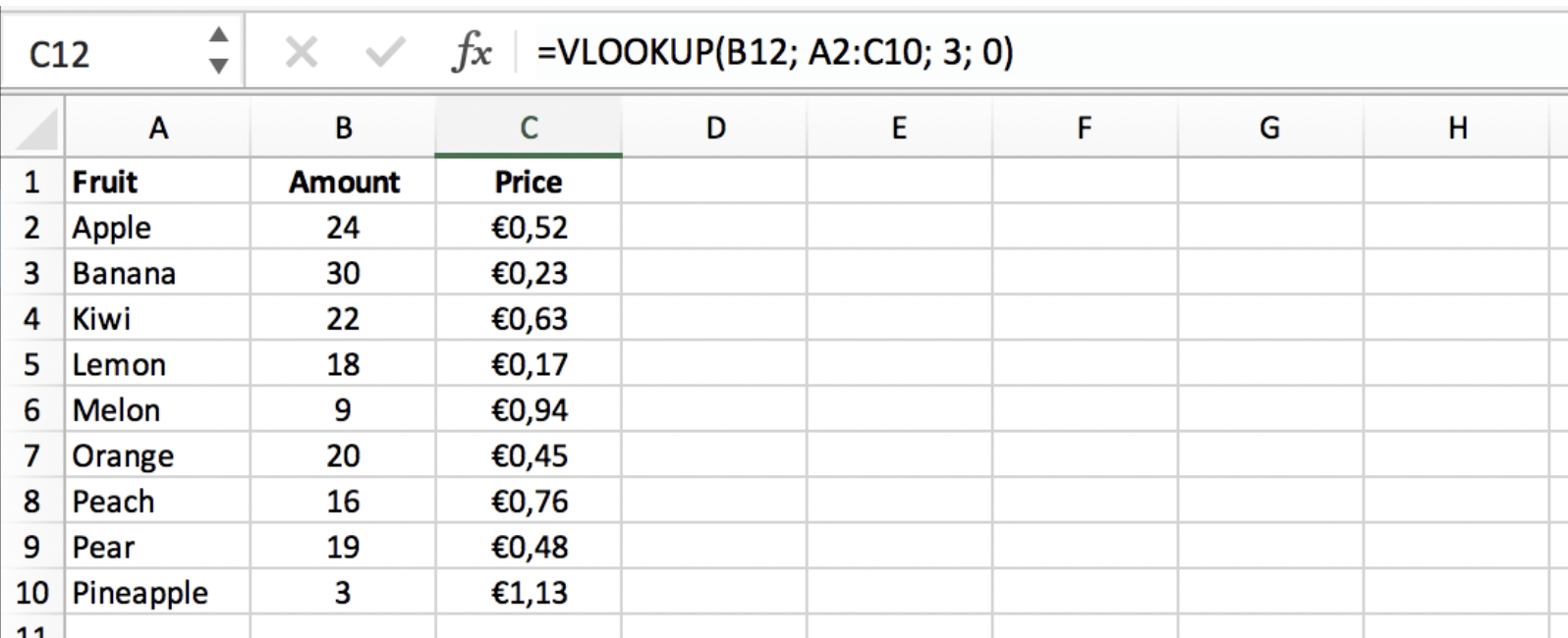
3. In the cell where you want to display the retrieved data, type the formula "=VLOOKUP(" and then select the cell containing the value you want to search for.
4. After selecting the search value, type a comma (,) to separate the arguments in the formula.
5. Select the range of cells in the table where you want to search for the value. This range should include the column with the search value and the column with the data you want to retrieve.
6. Type another comma (,) to separate the arguments.
7. Specify the column number in the table where the data you want to retrieve is located. Count the columns from left to right, starting with 1 for the leftmost column.
8. Type another comma (,) to separate the arguments.
9. Specify whether you want an exact match or an approximate match. Use "FALSE" for an exact match or "TRUE" or "1" for an approximate match. If you're not sure, use "FALSE" for now.
10. Close the formula with a closing parenthesis ")" and press Enter to calculate the result.
The VLOOKUP function will search for the specified value in the leftmost column of the table and return the corresponding value from the specified column. If a match is not found, the function will return an error or the closest approximate match if an approximate match was specified.You can then copy the formula to other cells to retrieve data for other values.
VLOOKUP is included in our Intermediate course here: https://go.courses/course/micrsoft-excel-intermediate-1-day